Gerry Tonkin-Hill

How many gene annotations are there?

Grace Blackwell recently gave a really interesting talk on her work Blackwell, G. A. et al. Exploring bacterial diversity via a curated and searchable snapshot of archived DNA sequences. Cold Spring Harbor Laboratory 2021.03.02.433662 (2021) doi:10.1101/2021.03.02.433662 generating a standardised and curated database of 661,405 bacterial genome assemblies using read data retrieved from the European Nucleotide Archive (ENA).

This dataset is already proving to be very useful. Grace has plans to generate gene annotations for the assemblies but was still deciding on the best approach for doing this in a standardised way across the very diverse dataset. We have run into this issue previously when developing panaroo. It is possible to force annotation algorithms like prodigal to use the same annotation model for each assembly. This helps to prevent the scenario where the exact same nucleotide sequence is annotated differently in separate genome assemblies. While this generates more standardised annotations it could repeatedly generate the same errors so it is unclear whether this is a preferable approach to allowing the algorithm to adapt to each genome individually.

⊕ One Two (xkcd)

In discussing this after her talk the question of how many possible annotations there are in a typical bacterial genome came up. As I did not have any intuition for this I thought it would be worth taking a quick look. Conveniently, prodigal has an output option -s that lists all possible annotations (after some rough filtering).

Taking a random S. pneumoniae, M. tuberculosis and K. pneumoniae genome assembly from the sets we used in the panaroo paper I ran prodigal using the -s option on each. I also ran the program excluding genes with N’s or that overlapped the ends of contigs to see how much impact these sources of error had.

1for f in *.fasta
2do
3prefix=$(basename $f .fasta)
4prodigal -i $f -o ${prefix}.gff -s ${prefix}_all.txt -f gff
5prodigal -i $f -o ${prefix}_filt.gff -s ${prefix}_filt_all.txt -f gff -c -m 
6done

We can then use a bit of python to count the number of annotations. I split this up to also count those that shared the same stop codon.

 1import glob
 2
 3counts = {}
 4for f in glob.glob('*_all.txt'):
 5  name = f.replace('_all.txt', '')
 6  annotations = []
 7  with open(f, 'r') as infile:
 8    for line in infile:
 9      if line[0] in ['#', 'B', '\n']: continue
10      line = line.split()
11      if line[2]=='-':
12        annotations.append((line[0], '-'))
13      else:
14        annotations.append((line[1], '+'))
15  counts[name] = [str(len(annotations)), str(len(set(annotations)))]
16  with open(name + '.gff', 'r') as infile:
17    count = 0
18    for line in infile:
19      if line[0]=='#': continue
20      count += 1
21  counts[name].append(str(count))
22
23with open('annotation_counts.csv', 'w') as outfile:
24  outfile.write('species,all,same_start,final\n')
25  for name in counts:
26    outfile.write(','.join([name]+list(counts[name])) + '\n')

We can then plot the final counts using ggplot

 1library(ggplot2)
 2library(data.table)
 3
 4counts <- fread("~/Downloads/annotation_counts.csv", data.table=FALSE)
 5counts$filtered <- ifelse(grepl('*filt', counts$species), 
 6                          'without closed ends', 'with closed ends')
 7counts$species <- gsub('_filt', '', counts$species)
 8plotdf <- melt(counts)
 9plotdf$species[grepl('k', plotdf$species)] <- 'K. pneumoniae'
10plotdf$species[grepl('s', plotdf$species)] <- 'S. pneumoniae'
11plotdf$species[grepl('tb', plotdf$species)] <- 'M. tuberculosis'
12
13ggplot(plotdf, aes(x=species, y=value, fill=species)) + 
14  geom_col() + 
15  facet_grid(variable~filtered) +
16  theme_minimal(base_size = 16) +
17  scale_y_sqrt(labels = function(x) format(
18    x, scientific = TRUE, digits=1, trim=TRUE),
19                     breaks = c(0,1e4,1e5)) +
20  theme(axis.title.x=element_blank(),
21        axis.text.x=element_blank(),
22        axis.ticks.x=element_blank()) +
23  xlab("") + ylab("annotation count")

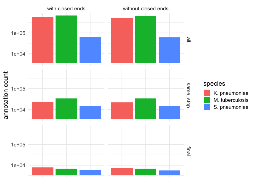
Overall it looks like there are around an order of magnitude more potential stop sites than the final list of genes output by prodigal. If we instead include the number of possible start sides for each stop site we find a further order of magnitude increase in the number of possible annotations. This is quite large and underscores the challenge of automatic gene annotation and the potential for small algorithmic decisions to have large consequences.

The exact number of annotations including those that overlap with contig ends is given in the following table.

Species	All	Same stop codon	Final
K. pneumoniae	234,325	31,006	5,791
M. tuberculosis	246,940	45,640	4,044
S. pneumoniae	74,255	17,242	2,184

Looking at the same table after excluding genes annotated at contig ends or across N’s we see that this has a small but not insignificant impact. In fact, we have previously found that the accumulation of these differences over many genomes can lead to large differences in pangenome inference.

Species	All	Same stop codon	Final
K. pneumoniae	220,963	30,463	5,351
M. tuberculosis	244,993	45,484	4,047
S. pneumoniae	73,552	17,163	2,147